Highlighting entire row based on cell value

This is if you want to highlight a complete row value based on cell value Let say we want to highlight all the applications which are tested i.e the  tested value is ‘yes’ 1) Select the entire group of cells. 2) go to conditional formatting and select ‘ Use formula to determine which cells to format 3) Enter the column value of the column which contains ‘yes’ as shown below

After adding rule we can choose the cells on which the conditional formatting is applicable.

This is what all the rows with value of ‘yes’ in their corresponding cells look like.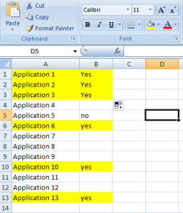

If you suddenly realize that the you want to change the value from ‘yes’ to ‘no’ simply change it. The highlighting on the row will automatically disappear.